Contents
- Index
Getting Started
Take an example the removal force values shown below. There is a lower spec limit of 4 pounds and upper spec limit of 15 pounds:

Start by entering the data in the first column of the Data window. The column labeled "Trans. Value" automatically displays the original values because no transformation has been selected.
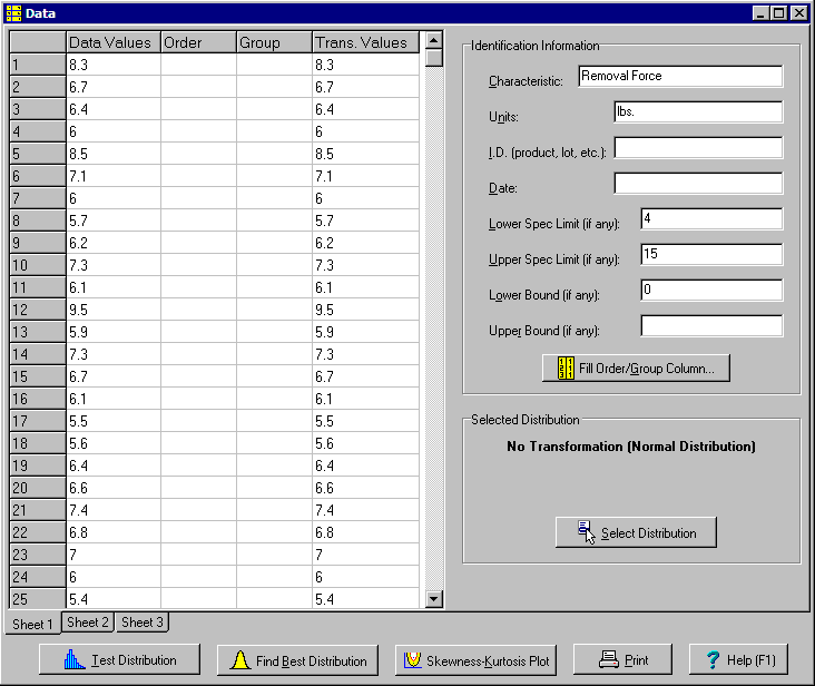
The Characteristic, Units, I.D. and Date fields are optional. Also enter any upper and lower spec limits. Finally enter any physical bounds. If negative values are impossible, there is a lower bound of zero. For yield data there is a lower bound of zero and upper bound of 100.
 Click the Test Distribution button to test whether the data fits the normal distribution and, if so, to perform additional analysis. The
 Test Distribution window appears as shown below:

A histogram of the data is shown along with estimates of the average, standard deviation, skewness and excess kurtosis. As no transformation was selected, the best fit normal curve is shown in blue.
Also shown are the results of the tests for normality. The first is a general test for all departures from normality called the Skewness-Kurtosis All test (SK All). This test has a p-value of 0.0199. A p-value of 0.05 or below results in failing the test. Because this test fails, one can state with 95% confidence that data is not from the normal distribution.
The second test for normality is the Skewness-Kurtosis Specific test (SK Spec). This test is designed to only reject for those departures from the normality that invalidate the confidence statements associated with normal tolerance intervals and variables sampling plans. Passing this test indicates it is OK to use these two procedures even if the other normality test fails. As this test also fails, the data is not normal in a manner than does not allow these two procedures to be used. As a result, no further analysis is performed. The data must first be transformed. Pp and Ppk are also shown, but care must be taken in interpreting these values. The relationship commonly provided between these values and the defect level depends on normality.
 Click the Find Best Distribution button to determine which distribution best fits the data. For every distribution there is a transformation that makes the transformed values fit the normal distribution so finding the best fit distribution is the same as finding the best transformation. In this case, the best fit distribution is described as the Johnson Distribution (6.667489, 1.049613, 2.048305, 11.284237). The values given after the name of the distribution are the parameters of the distribution represented as the average, standard deviation, skewness and kurtosis.
Next click the Test Distribution button again to see if the Johnson distribution fits the data. The results are shown below:
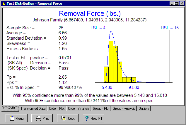
This time both tests pass. The Johnson distribution fits the data and can be used to analyze and transform the data. The Johnson distribution fit to the data is shown in blue. As a result, further analysis is performed and shown at the bottom. The resulting tolerance interval is: "With 95% confidence more than 99% of the values are between 5.143 and 15.610." The resulting variables sampling plan gives: "With 95% confidence more than 99.341% of the values are in spec." The confidence level and percent in the interval can be adjusted using the Analysis Options and Tolerance Interval Options dialog boxes.
It may have originally been desired to demonstrate with 95% confidence 99% of the product is in spec. A common approach is to use a normal tolerance interval that has 95% confidence of containing 99% of the values. If this interval is within the spec limits, the criteria is demonstrated to have been meet. In the above example, the normal tolerance interval is outside the specs and thus fails. A second approach is to use a variables sampling plan. This results in the second statement, which passes. These two approaches frequently agree but in a small number of cases, the variables sampling plan will pass when the normal tolerance interval fails. This is because the normal tolerance interval constructs one interval containing 99% of the values, but it is not the only such interval that can be constructed. The displayed interval is constructed based of 0.5% falling out each end. Other intervals can be constructed such as with 0.25% outside the lower end and 0.75% outside the upper end. One of these tolerance intervals might be inside the spec limits and pass.
To further understand the transformation and how it works, the second tab of the Test Distribution window shows the transformation:

The transformation equation, in EXCEL format, is shown at the top:
= -7.40839397009538 + 1.78277265296386 * ASINH((X - 4.94211049770679) / 0.0462347042237263)
A histogram of the transformed values is shown along with the best fit normal curve. The same transformation is applied to the spec limits as well. The transformed values themselves are shown in the last column of the Data window.
The Ppk, Pp, percent in spec, tolerance interval and confidence statement relative to the spec limits are all calculated using the transformed values. These same results were displayed on the previous page except the tolerance interval (-3.528, 3.528) is transformed back into the original units of measure (5.143, 15.610) by applying the inverse of the transformation equation. From the above analysis, it is seen more values are predicted to exceed the upper spec limit than the lower.
Distribution Analyzer will also:
Test for shifts over time if the order the data points were collected is indicated in the Order column of the Data window.
Test for differences between groups like cavities, nozzles and operators if the groups are indicated in the Group column of the Data window.
Identify potential outliers.
Generate random values.
Understand relationships between distributions using a Skewness-Kurtosis plot.
Further help getting started can be found in the user manual at http://www.variation.com/da.